For years now, I have been making these small projects
(8 years since the first one!, geesh, I'm old), Here are some of them:
- A face-centering gimballed Camera mounted on RPI
- A hand-motion controlled DJI Tello Drone
- At times, I use these projects to learn new stuff (whether work-related or just for fun):
Intro
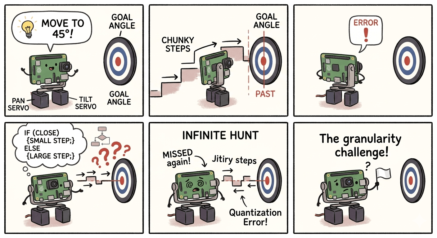
During my first one, an RPI-powered gimbal, I hit an uncanny snag: The movement was painfully 'chunky.' Instead of a smooth sweep, the camera moved in awkward, rigid increments. Setting a target angle triggered a frustrating loop
— The servos would leap toward the goal, but because their fixed step size was larger than the remaining error, they’d overshot it every time.
I tried to outsmart the hardware with a series of 'if-else' statements to shrink the steps as the camera closed in, but the result was the same. The system was trapped in an infinite hunt, perpetually jumping back and forth across a target it lacked the granularity to actually hit:
Essentially - doing this:
So I asked a dear friend about this, and he asked:
Have you heard of PID?
[Wikipedia]
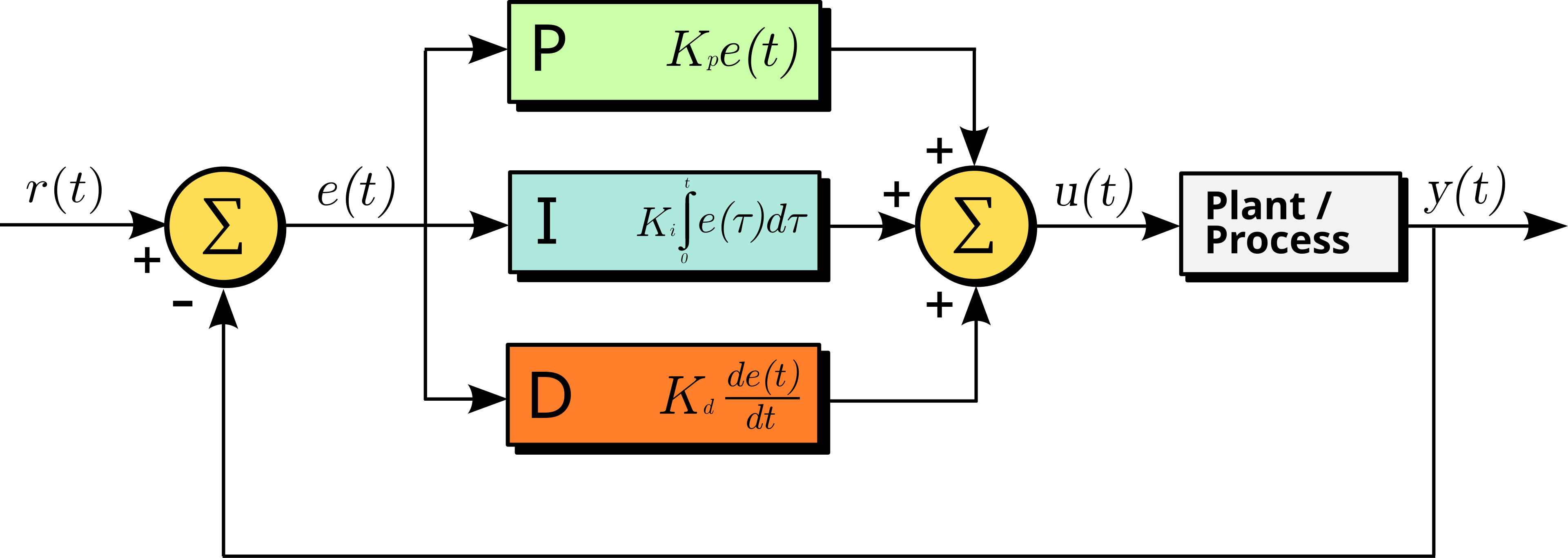
A proportional–integral–derivative controller (PID controller or three-term controller) is a feedback-based control loop mechanism commonly used to manage machines and processes that require continuous control and automatic adjustment. It is typically used in industrial control systems and various other applications where constant control through modulation is necessary without human intervention. The PID controller automatically compares the desired target value (setpoint or SP) with the actual value of the system (process variable or PV). The difference between these two values is called the error value, denoted as e(t).
Fast forward from 2019, decades ago in a "Pre-LLM" era. At the time, the math behind PID controllers was a hard "no" for me. Yet, those jagged, step-like movements kept appearing in every project.
At its core, control theory is just the art of error minimization, and it's definitely not limited to robotics. I’ve had "Learn PID" sitting on my Udemy wishlist for years with a "one day, Gal" sticky note attached...
Seven Years later
Lately, I’ve been diving deep into the world of control theory via Udemy's Applied Control Systems 1: autonomous cars: Math + PID + MPC. Between the chaotic energy of raising two toddlers, navigating the day job’s endless stream of charts, and the midnight ritual of folding laundry, finding "deep work" time is a challenge—but the payoff has been worth the grind.
One of the first modules in the course involves building a PID-controlled water tank simulation. The objective is straightforward: automate the filling and emptying of a tank to maintain a specific setpoint within a controlled environment.
(While the course used Python for its examples, I naturally opted to write it in C++ and OpenCV)
This is the water-tank simulation (watch with subtitles turned on):
Breaking Down the PID Logic
At its core, this simulation addresses a classic 1-dimensional PID problem. It’s a good and simplified example observing how the Proportional, Integral, and Derivative gains interact to minimize steady-state error and manage overshoot in a dynamic system.
Creating a water-tank simulation was fun, but it wasn't as near as building a robot that is controlled by a PID controller!
Although the course is pure PID concept, it doesn't require knowledge of ROS (nor Gazebo). Yet I'm a total nerd, so why not...
Controlling a Tracked Vehicle in Gazebo SIM using ROS2
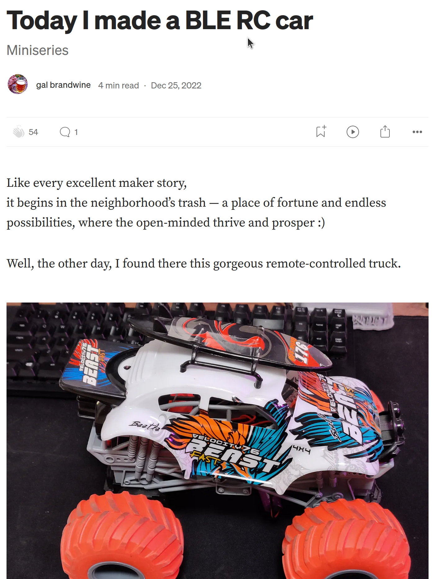
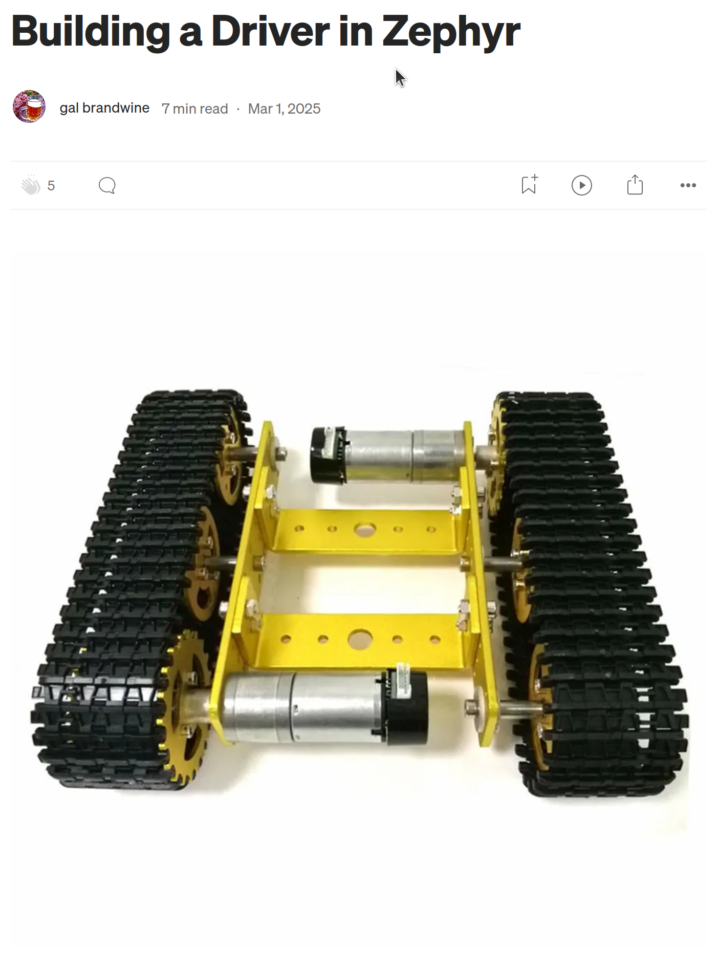
A while back, I bought a Tank chassis from Aliexpress. I used it to learn Zephyr, and its Generic Driver API -
Once completed;
Plan A was to mount Ultrasonic sensors on it. Then life happened, and the time required for hardware debugging became hard to find. So, the next best thing for me was to simulate stuff using Gazebo & ROS2.
Gazebo, which provides the heavy lifting for the simulation, while ROS2 handles the PID logic. It’s the perfect way to scratch that robotics itch when you only have a spare hour to sit down and code.
Gazebo
Gazebo - is an open-source 3D robotics simulator that enables accurate modeling, simulation, and testing of robots in complex indoor and outdoor environments.
It provides high-fidelity physics simulation, rendering, and sensor data generation to test algorithms, control strategies, and hardware configurations safely before physical deployment, often integrated with ROS
Modeling the Tank chassis using Gazebo's SDF took some time (mostly understanding Gazebo's collision concepts - which describe how parts collide with each other) - Luckily, here's where Gemini came to the rescue.
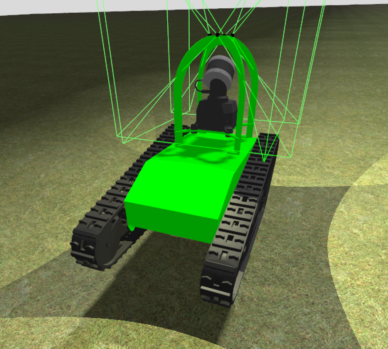
For starting point, I've downloaded from Gazebo-OpenRobotics a model of a tracked vehicle:
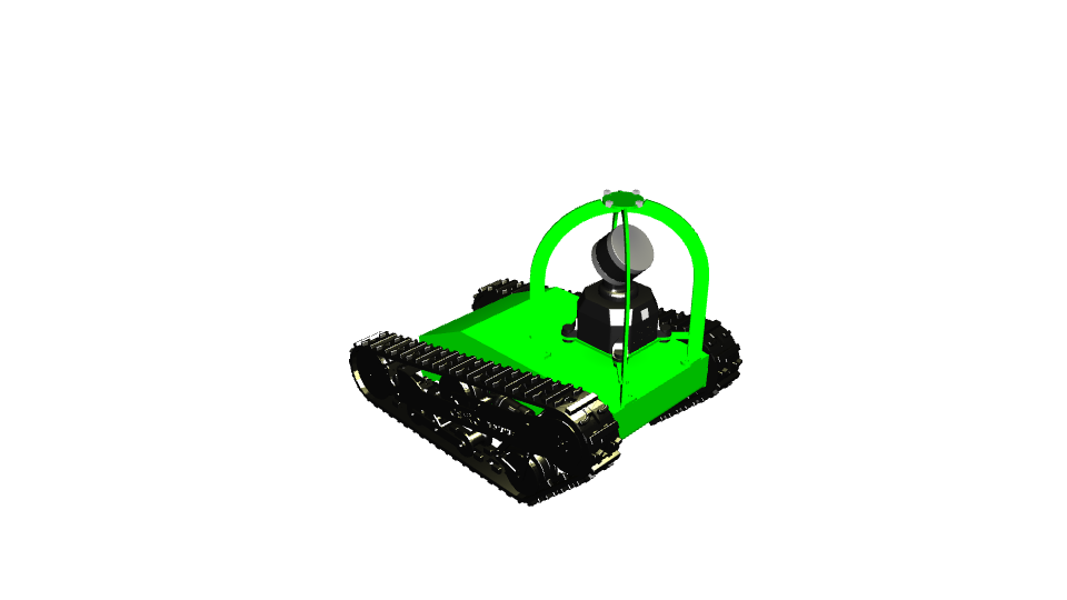
Tailored its SDF [Simulation Description Format] file to match my needs, and loaded it into one of Gazebo's default map: heightmap.
Running it all together was simple and friendly:
(Operating within a container)
Terminal 1:
# Telling Gazebo where to find my model
export GZ_SIM_RESOURCE_PATH=/home/pid_user/ros2_examples/src/gazebo/models:$GZ_SIM_RESOURCE_PATH

# Then run Gazebo pointing to the heightmap I've downloaded:
gz sim ./ros2_examples/src/gazebo/models/heightmap.sdf
Terminal 2:
# Driving Forward
gz topic -t /model/csiro_data61_dtr_sensor_config_2/cmd_vel -m gz.msgs.Twist -p "linear: {x: 0.5}, angular: {z: 0.0}"
While designing how I will control it, I faced a few options for controlling the tracked vehicle.
- Either control each tracker
- Or control them both as one
For simplicity, I opted for the latter, using Gazebos TrackedVehicle plugin, which accepts a message of type Twist with the following data:
linear: {x: 0.5},
angular: {z: 0.0}
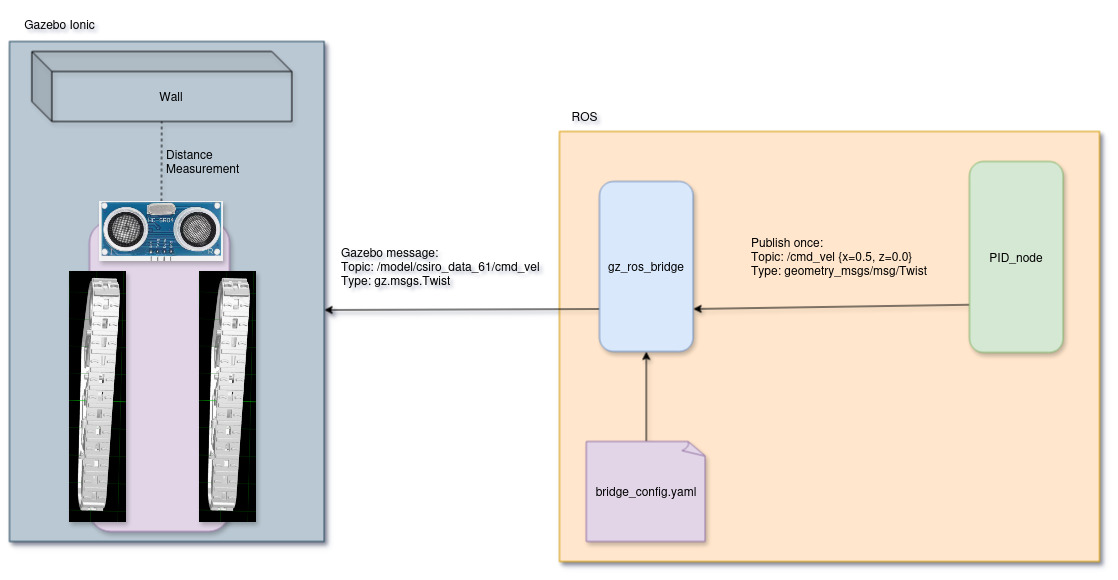
Connecting Gazebo with ROS2
I want my PID to live inside a ROS2 node; luckily, ROS2 is packed with a gz_ros_bridge tool, which translates Gazebo messages to ROS2's.
Rosbridge supports a simple mapping approach, which includes topics going out/in:
# Control the vehicle from ROS 2
- ros_topic_name: "cmd_vel"
  gz_topic_name: "/model/csiro_data_61/cmd_vel"
  ros_type_name: "geometry_msgs/msg/Twist"
  gz_type_name: "gz.msgs.Twist"
  direction: ROS_TO_GZ

# Get odometry data back to ROS 2
- ros_topic_name: "odom"
  gz_topic_name: "/model/csiro_data_61/odometry"
  ros_type_name: "nav_msgs/msg/Odometry"
  gz_type_name: "gz.msgs.Odometry"
  direction: GZ_TO_ROS

# Get the clock (essential for TF and Nav2)
- ros_topic_name: "clock"
  gz_topic_name: "/world/heightmap/clock"
  ros_type_name: "rosgraph_msgs/msg/Clock"
  gz_type_name: "gz.msgs.Clock"
  direction: GZ_TO_ROS

  # Get distance sensor data back to ROS 2
- ros_topic_name: "front_scan"
  gz_topic_name: "/front_distance"
  ros_type_name: "sensor_msgs/msg/LaserScan"
  gz_type_name: "gz.msgs.LaserScan"
  direction: GZ_TO_ROS

# Pack here more topics to bridge
And call:
ros2 run ros_gz_bridge parameter_bridge --ros-args -p config_file:=bridge_config.yaml
From this moment on, Gazebo and ROS2 are streamlined,
I can now use RViz2 \ RQT for visualization, and ROS nodes for communication with the Gazebo sim.
Here's a small sanity check [On the right: ROS's RQT, on the left: Gazebo]:
Now I need to write a ROS Node operating this tank.
Let's get to it!
ROS2
ROS is great for encapsulating my PID and logic.
For Starters, I'll play with a simple ROS2 Node that moves the TrackedVehicle forward, without any feedback loop:
I'll add some minimal C++ examples from now on
#include <chrono>
#include <memory>
#include <string>

#include "rclcpp/rclcpp.hpp"
#include "geometry_msgs/msg/twist.hpp"

using namespace std::chrono_literals;

class CmdVelPublisher : public rclcpp::Node
{
public:
  CmdVelPublisher()
      : Node("cmd_vel_publisher")
  {
    // Create the publisher on the "cmd_vel" topic
    publisher_ = this->create_publisher<geometry_msgs::msg::Twist>("cmd_vel", 10);

    timer_ = this->create_wall_timer(
        1s, std::bind(&CmdVelPublisher::timer_callback, this));

    feature_future_ = feature_promise_.get_future().share();

    RCLCPP_INFO(this->get_logger(), "C++ CmdVel Publisher has started.");
  }

  std::shared_future<void> get_feature_future() const
  {
    return feature_future_;
  }

private:
  void timer_callback()
  {
    // Fire this timer only once
    this->timer_->cancel();

    auto message = geometry_msgs::msg::Twist();

    // Set forward velocity (m/s)
    message.linear.x = 0.5;

    // Set angular velocity (rad/s)
    message.angular.z = 0.0;

    RCLCPP_INFO(this->get_logger(), "Publishing: Linear='%f'", message.linear.x);
    publisher_->publish(message);

    // Complete the feature once the message is published.
    try
    {
      feature_promise_.set_value();
    }
    catch (const std::future_error &e)
    {
      RCLCPP_WARN(this->get_logger(), "Future exception: %s", e.what());
    }
  }

  rclcpp::TimerBase::SharedPtr timer_;
  rclcpp::Publisher<geometry_msgs::msg::Twist>::SharedPtr publisher_;
  std::promise<void> feature_promise_;
  std::shared_future<void> feature_future_;
};

int main([[maybe_unused]] int argc, [[maybe_unused]] char **argv)
{
  rclcpp::init(argc, argv);

  auto node = std::make_shared<CmdVelPublisher>();
  rclcpp::executors::SingleThreadedExecutor exec;
  exec.add_node(node);
  exec.spin_until_future_complete(node->get_feature_future());
  rclcpp::shutdown();
  return 0;
}
The ROS2 Node above wakes up, fires a Twist message — a standard ROS structure containing linear and angular velocity commands — on the /cmd_vel topic, and then shuts down.
Gradually overloading the example toward PID.
The code below shows an example of a simple closed-loop controller that does as follows:
- Subscribe to front-distance-scans
- Publish
move forward at 5.0[m/s] - When distance is < 0.5[m] - Publish Stop
Using this code example, I simulate an overshooting problem.
#include <chrono>
#include <memory>
#include <string>

#include "rclcpp/rclcpp.hpp"
#include "geometry_msgs/msg/twist.hpp"
#include "sensor_msgs/msg/laser_scan.hpp"
#include "std_msgs/msg/float32.hpp"

using namespace std::chrono_literals;

class VehicleCtrlCloseLoop : public rclcpp::Node
{
public:
    VehicleCtrlCloseLoop()
        : Node("vehicle_ctrl_close_loop_velocity")
    {
        RCLCPP_INFO(this->get_logger(), "Initializing Node: %s", this->get_name());
        // Define QoS: sensor data typically uses SensorDataQoS (Best Effort)
        auto qos = rclcpp::SensorDataQoS();

        m_wall_distance_subscriber = this->create_subscription<sensor_msgs::msg::LaserScan>("front_scan", qos, [&](const sensor_msgs::msg::LaserScan::SharedPtr msg)
                                                                                            { this->new_distance_measurement_cb_(msg); });

        // Create the publisher on the "cmd_vel" topic
        m_publisher = this->create_publisher<geometry_msgs::msg::Twist>("cmd_vel", 10);

        m_debug_new_measurement_publisher = this->create_publisher<std_msgs::msg::Float32>("/pid/debug/wall_distance/new", qos);
        m_debug_target_publisher = this->create_publisher<std_msgs::msg::Float32>("/pid/debug/wall_distance/target", qos);

        feature_future_ = feature_promise_.get_future().share();

        RCLCPP_INFO(this->get_logger(), "C++ vehicle_ctrl_open_loop Node has started.");
    }

    std::shared_future<void> get_feature_future() const
    {
        return feature_future_;
    }

private:
    void new_distance_measurement_cb_(const sensor_msgs::msg::LaserScan::SharedPtr newScan)
    {

        // Wait for first distance measurement.
        if (!is_published)
        {
            this->move_forward(5.0f);
            is_published = true;
        }

        auto front_distance = newScan->ranges[0];

        // Debug messages
        auto new_measurement_msg = std_msgs::msg::Float32();
        new_measurement_msg.data = front_distance;
        m_debug_new_measurement_publisher->publish(new_measurement_msg);

        auto desired_distance_from_wall_msg = std_msgs::msg::Float32();
        desired_distance_from_wall_msg.data = 0.5;
        m_debug_target_publisher->publish(desired_distance_from_wall_msg);

        if (front_distance < 0.5)
        {
            move_forward(0.0);
            this->set_future(); // Trigger roshutdown
        }
    }

    void move_forward(const float forward_velocity)
    {

        auto message = geometry_msgs::msg::Twist();
        message.linear.x = forward_velocity; // Set forward velocity (m/s)
        message.angular.z = 0.0;             // Set angular velocity (rad/s)
        m_publisher->publish(message);
    }

    /// @brief Complete the feature once the message is published.
    void set_future()
    {
        try
        {
            feature_promise_.set_value();
        }
        catch (const std::future_error &e)
        {
            RCLCPP_WARN(this->get_logger(), "Future exception: %s", e.what());
        }
    }

    rclcpp::TimerBase::SharedPtr timer_;
    rclcpp::Subscription<sensor_msgs::msg::LaserScan>::SharedPtr m_wall_distance_subscriber;
    rclcpp::Publisher<geometry_msgs::msg::Twist>::SharedPtr m_publisher;
    rclcpp::Publisher<std_msgs::msg::Float32>::SharedPtr m_debug_new_measurement_publisher;
    rclcpp::Publisher<std_msgs::msg::Float32>::SharedPtr m_debug_target_publisher;
    std::promise<void> feature_promise_;
    std::shared_future<void> feature_future_;
    bool is_published{false};
};

int main([[maybe_unused]] int argc, [[maybe_unused]] char **argv)
{
    rclcpp::init(argc, argv);

    auto node = std::make_shared<VehicleCtrlCloseLoop>();
    rclcpp::executors::SingleThreadedExecutor exec;
    exec.add_node(node);

    RCLCPP_INFO(node->get_logger(), "Waiting for cmd_vel publish to complete feature...");
    exec.spin_until_future_complete(node->get_feature_future());

    RCLCPP_INFO(node->get_logger(), "Feature complete: cmd_vel has fired once.");

    rclcpp::shutdown();
    return 0;
}
Here's the recording:
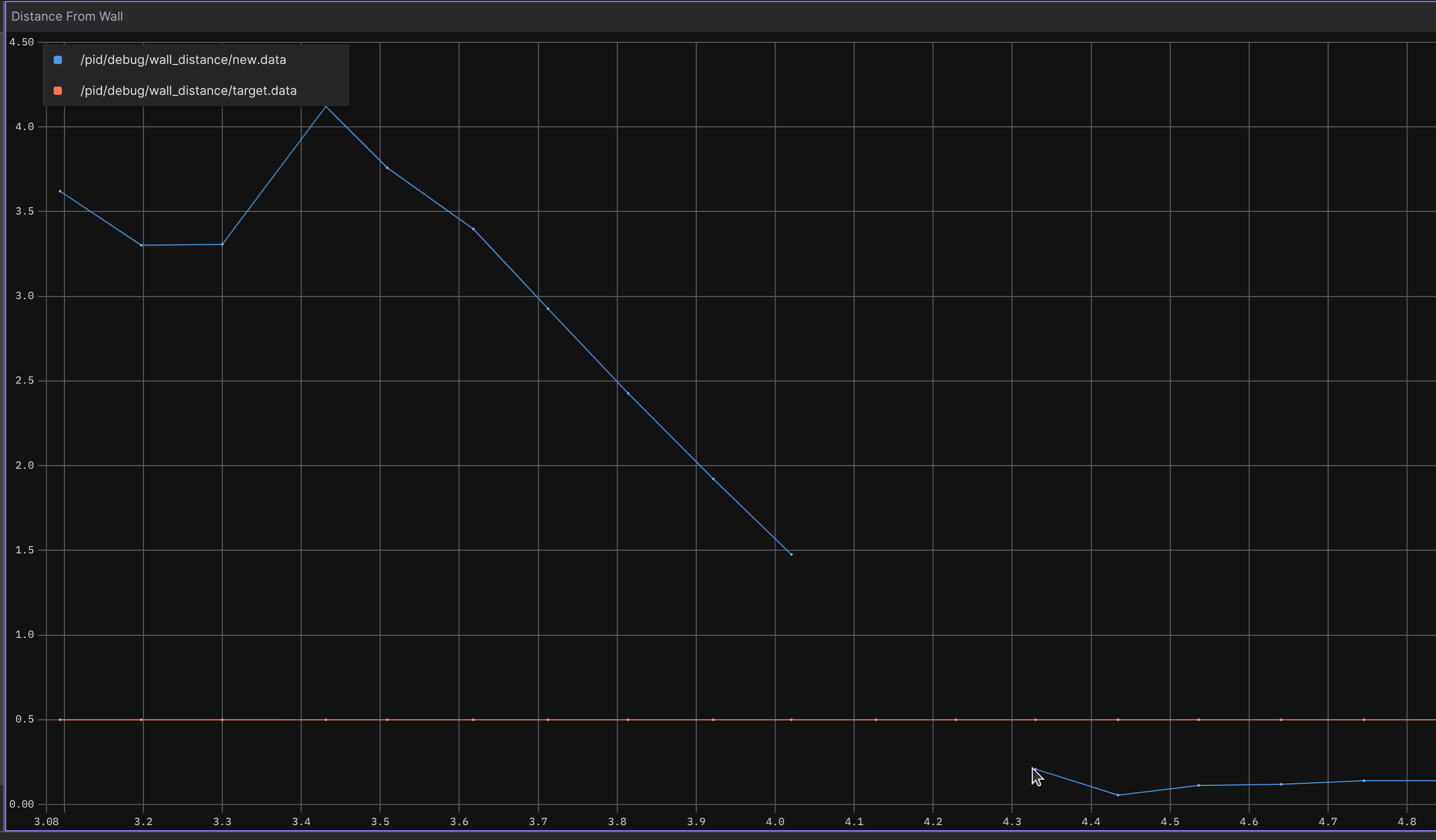
- The blue dots - new distance measurements (at 10[hz])
- The orange dots - desired distance (I want the vehicle to stop 0.5[m] before the wall)
We can notice two things:
1. The slope of the blue line is linear, which means the vehicle is getting closer to the wall at the same speed as it was in the previous sample, which means the vehicle is not slowing down toward the target.
2. The vehicle is missed by $0.3[m]$ of the desired target (the left-most blue dot under the orange line).
From what I've gathered so far, in Control Systems Theory, we affect the system by changing its state. Our state is defined as `distance from the wall`, i.e, distance $x[m]$ measured by a sensor. Our input to the system is $v[m/s]$, calculated by the controller.
Essentially:
1. We know sensor sampling frequency - for every sampling cycle, we get a new distance_measurement. This is our $dt$
2. $x_t(i) = \text{new-distance-measurement of time } i$
3. Our error looks like this: $e_t = \frac{x_t(i) - x_t(i-1)}{dt}$
And with a small reminder from physics, that velocity can be calculated as follows:
We can understand that $v$ is our new input to the system. And this velocity needs to slow down as the vehicle approaches the target (also known as the reference).
The P of the PID
The P part usually controls the size of the steps we are going to take towards our target. As mentioned above, the steps in our systems are $v[m/s]$ of time $t[s]$. Essentially, we need to send smaller and smaller velocity commands.
Looking at the example above, the controller for every new measurement essentially does this:
if measured_distance < target_distance:
    move_forward(0.0f) # Stop
When considering the measurement frequency, the vehicle speed, the vehicle mass, and probably more variables. Chances for stopping exactly at the target_distance are pretty low.
Hence, we want our velocity to change in proportion to our distance:
error = new_measured_distance - reference # Error will get smaller as the vehicle get closer
new_velocity = kP*error
move_forward(new_velocity)
kP - is used for various reasons:
Dimensional Alignment
My Error is in meters, but the system Output must be in meters per second.
Without Kp, we are saying: "For every 1 meter of distance error, I want 1 m/s of speed."
This 1:1 ratio is arbitrary. What if your robot is a massive 50-ton tank? Or a tiny 100-gram drone?
Kp defines the scaling factor.Control The "Aggression" Level
Kp determines how hard the system fights to correct the error.
Low Kp (e.g., 0.1): The robot is "lazy." It sees a 2-meter error and crawls at 0.2 m/s. It is very stable and won't overshoot, but it might never reach the target if there is a tiny bit of friction or a ramp.
High Kp (e.g., 10.0): The robot is "aggressive." It sees a 2-meter error and tries to launch at 20 m/s. It will reach the target fast, but it will likely slam into the wall because it has too much momentum to stop.
Theoretically, the vehicle is moving forward, so new_measurement is getting closer to target -> minimizing the error.
Respecfully, new_velocity is getting smaller:
We can see exactly this from recordings:
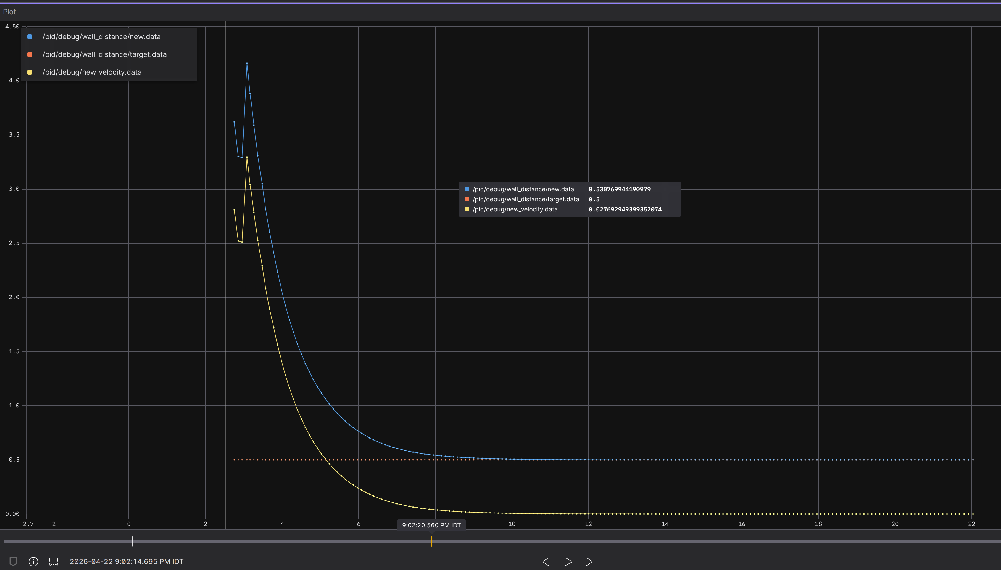
Observe how new_velocity is being reduced as the tracked-vehicle gets closer to the target (blue line meets orange).
Well, you might've thought, That looks perfect, why continue? - lets learn more!
The I of the PID
Motivation:
The thing is with Proportional controllers, that they don't have an integral part. So eventually they correlate with the current measurement.
(the way I see it - they don't have memory of previous states).
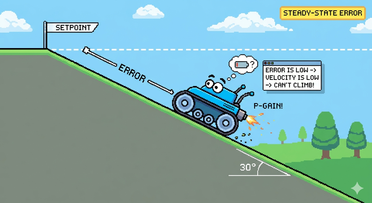
Navigating an uphill gradient introduces a classic control challenge: the 'near-miss' stall. As the vehicle nears the wall, the controller scales back velocity commands to a crawl. On an incline, these outputs often become too weak to fight gravity, leaving the vehicle stuck just short of the goal. By implementing the Integral action, we ensure the controller 'recognizes' this persistent error and ramps up the torque necessary to close the final gap.
Thats called Steady-state error: The difference between the target and the actual position once the system stabilizes. This is a cute genai giff trying to represent it:
I is the controller's integrator, it integrates the error over time.
As a reminder, here's the full PID controller mathematical representation:
The Integral component specifically focuses on accumulation:
In the C++ implementation, I use a discrete summation:
This is how my PI controller looks (pasting only the callback of new distance-measurement):
void new_distance_measurement_cb_(const sensor_msgs::msg::LaserScan::SharedPtr newScan)
{
    // Wait for first distance measurement.
    if (!is_published)
    {
        is_published = true;
        m_prev_time = this->get_clock()->now();
    }

    auto new_measurement = newScan->ranges[0];
    float reference = 0.5f; // Desired distance from the wall

    // Calculate dt:
    // Inside a node callback
    rclcpp::Time now = this->get_clock()->now();
    double dt = (now - m_prev_time).seconds(); // Remember - My system is outputting velocity - which is measured in m/s units. So I need to stay in the Seconds domain
    m_prev_time = now;

    // ERROR CALCULATION: No fabs(). Must be signed.
    auto de_t = new_measurement - reference;

    // Derivative Calculation
    auto derivative = 0.0f;
    // Skip the first two samples, so dt could be a real number
    if (m_num_messages_received > 2)
    {
        derivative = (de_t - m_prev_error) / static_cast<float>(dt);
        m_prev_error = de_t;
    }

    // INTEGRAL ACCUMULATION I = \integral(de(t)*dt)
    // Unit: Meter-Seconds
    m_I += de_t * static_cast<float>(dt);

    // Integral Windup
    if (m_I > 1.0f)
        m_I = 1.0f; // Example clamp
    if (m_I < -1.0f)
        m_I = -1.0f;

    // New System Input
    auto new_velocity = (m_kP * de_t) + (m_kI * m_I) + (m_kD * derivative);


    move_forward(new_velocity);
    m_num_messages_received++;
}
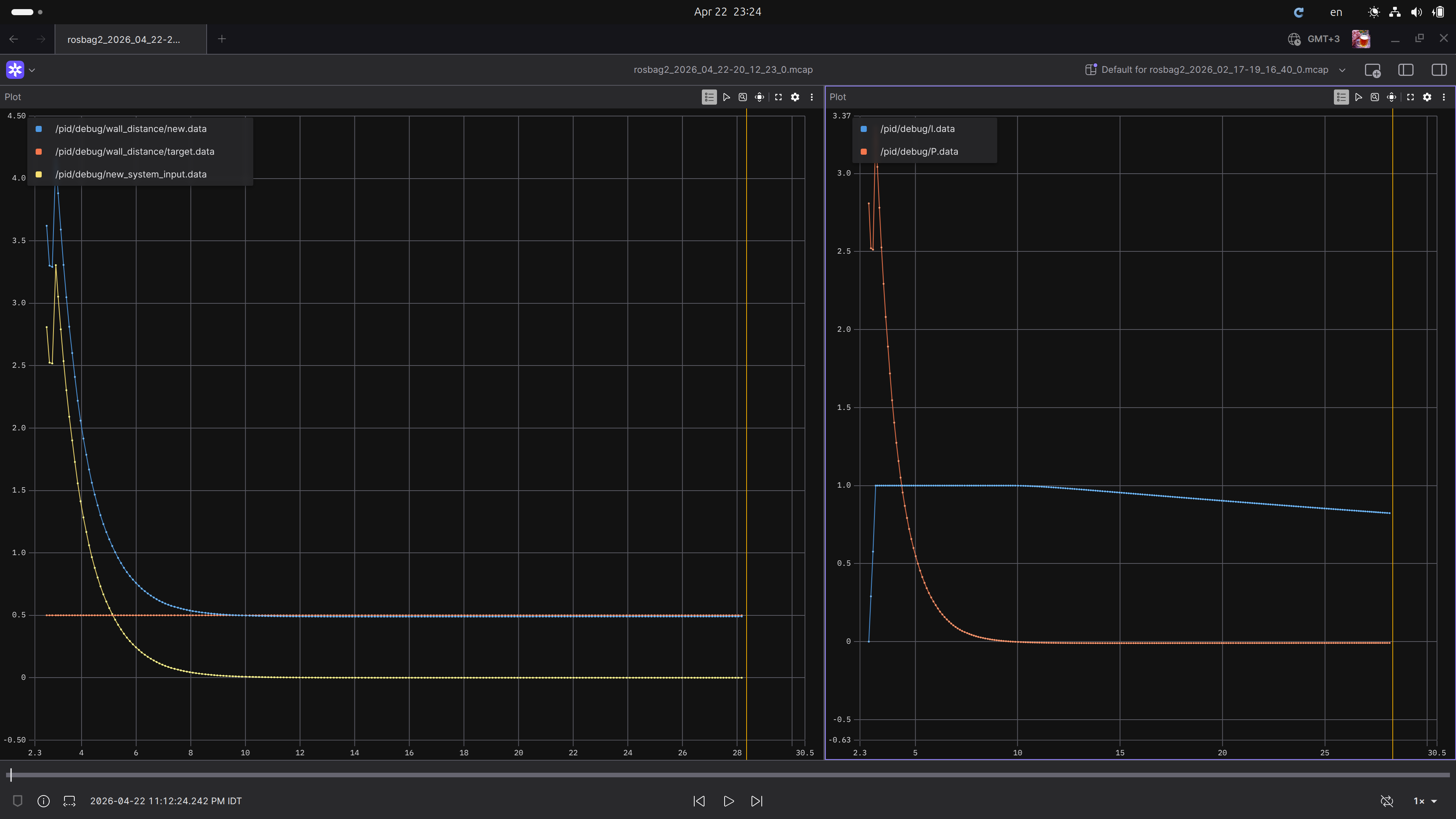
Looking at the data from the simulation, something strange happened:
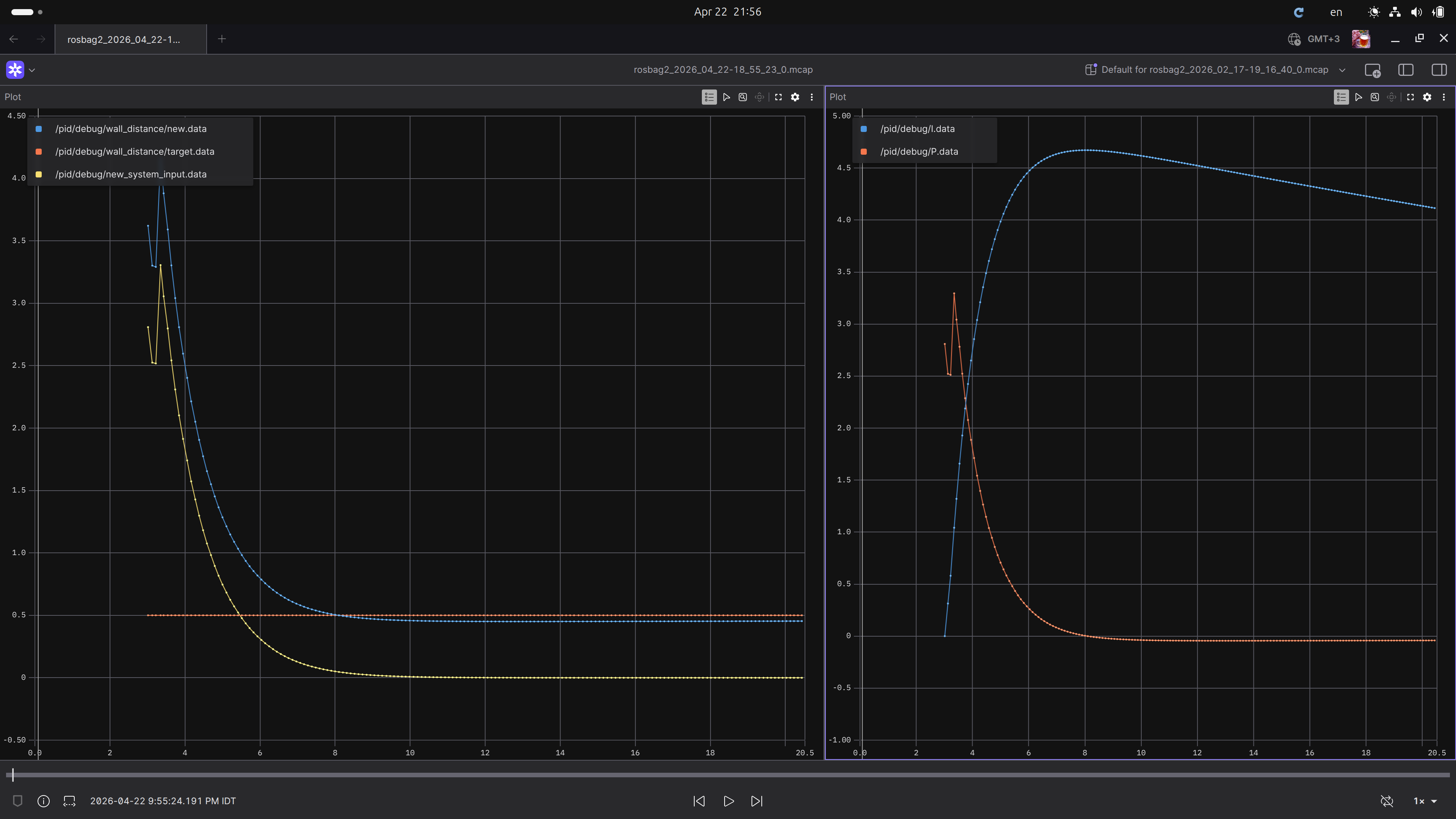
Here's what is going on in this recording:
PID coefficients: $kP=0.9, kI=0.01$
1. The error is large $\rightarrow$ the vehicle starts moving at high velocity
2. The Integrator is summing up all the large errors
3. The vehicle overshoots the desired target [orange line]$\rightarrow$ $P$ immediately changes sign to negative, minimizing the error back to $0$
4. By this time, $I$ gained too much "memory mass" of a `positive` error $\rightarrow$ so the $K_I\cdot{I}$ part is much larger than the $K_p\cdot{e(t)}$ part of the PI controller $\rightarrow$ the `new velocity` (our new_system_output) is slowly changing its sign from positive to negative - only then, the vehicle will start going backwards.
There are two things here:
1. Clearly kI is too small - it merely affectsI.
2. The Integrated part of the PI controller is gaining too much "error memory mass." Up to a point, the tracked vehicle overshoots the desired distance, but it looks like it kept its own margin
In the following recording, I've increased kI to 0.1, see how it affected:
PID coefficients: kP=0.9, kI=0.1
With larger kI, the error is being minimized much faster!
the error integration; $K_i \int_{0}^{t} e(t)dt$ is getting larger.
Eventually pulling toward the target, even if the vehicle is trying to slow down!
Although this caused even larger overshooting, we can see that the error is minimized eventually to the desired target.
Now, regarding the second bullet The Integrated part of the PI controller is gaining too much "error memory mass." (This is called Integral Windup):
There's a simple solution for that, called Integral windup. According to Wikipedia. This problem can be addressed by:
- Initializing the controller integral to a desired value, for instance, to the value before the problem[citation needed]
- Increasing the setpoint in a suitable ramp
- Conditional integration: disabling the integral function until the to-be-controlled process variable (PV) has entered the controllable region
- Preventing the integral term from accumulating above or below pre-determined bounds
- Back-calculating the integral term to constrain the process output within feasible bounds.
- Clegg integrator: Zeroing the integral value every time the error is equal to, or crosses zero. This avoids having the controller attempt to drive the system to have the same error integral in the opposite direction as was caused by a perturbation, but induces oscillation if a non-zero control value is required to maintain the process at the setpoint.
Trying the Preventing Integrating outside pre-determined bounds approach, by simply adding to my callback:
// 3. Integral with Clamping (Anti-Windup)
    m_I += de_t * static_cast<float>(dt);
    if (m_I > 1.0f) m_I = 1.0f;       // Example clamp
    if (m_I < -1.0f) m_I = -1.0f;
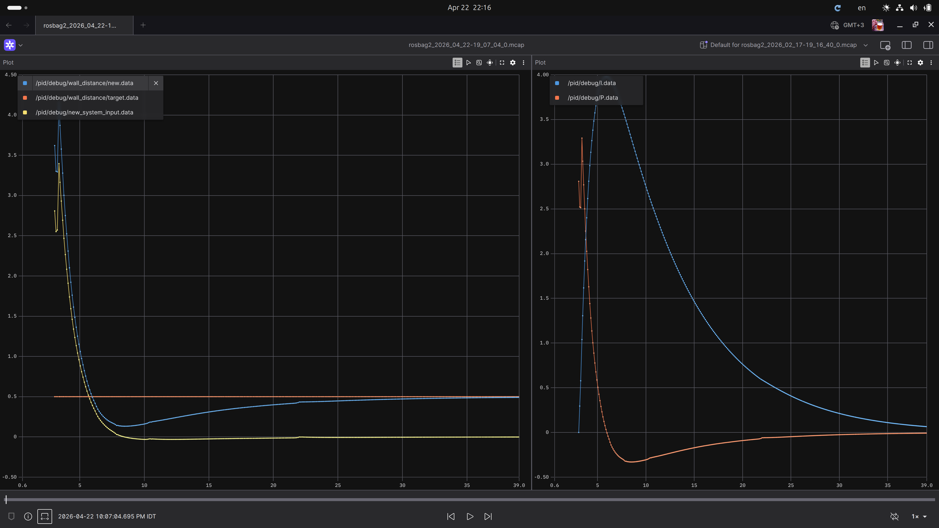
Here's what my Integral Windup looks like from the recordings:
We can see two things above:
1. There's no overshoot - because when the error is too large, the velocity is controlled mostly by the Proportional part.
2. The calmping of the Integral (the blue in the right) - the Integrated section does not gain memory when outside of its thresholds
Although Im curisoue cheking the Clegg integrator approach for Integral-windup. I continue with the final part of the PID controller:
The D of the PID
Another reminder, here's the full PID controller mathematical representation:
I've covered the Proportional part $K_p e(t)$ - where it reduces the system-input (in my case, velocity) in proportion to the error
The Integral part $K_i \int_{0}^{t} e(t) dt$ - where it has "memory", and integrates the errors to prevent Steady State Error
Now we get to The Derivative — which is essentially the "Brakes" or the "Fortune Teller" of the system.
Why do we need it? [LLM answer ahead!]
If P is the muscle and I is the persistence, D is the dampener.
Predicting the Future: The D-term looks at how fast the error is shrinking. If the error is decreasing very rapidly (meaning the tracked-vehicle is racing toward the wall), the D-term becomes a large negative value. It "predicts" that you’re about to overshoot and starts pushing back before you even hit the target.
Preventing Overshoot: Remember your graph where the vehicle overshot the orange line and then had to come back? That happened because the vehicle had too much momentum. The D-term acts like a shock absorber, slowing the vehicle down as it gets closer so it "lands" softly on the setpoint.
Counteracting Oscillations:
Without D, a high-gain P controller will make the vehicle bounce back and forth across the target forever. D adds "friction" to the control signal to stop that bouncing.
To complete my PID controller, I'll expand my CPP callback with a derivative calculation on the error:
double derivative = (current_error - previous_error) / dt;
double D_out = Kd * derivative;
And the final PID controller (it's completely implemented in the callback function):
void new_distance_measurement_cb_(const sensor_msgs::msg::LaserScan::SharedPtr newScan)
{
    // Wait for first distance measurement.
    if (!is_published)
    {
    is_published = true;
    m_prev_time = this->get_clock()->now();
    }

    auto new_measurement = newScan->ranges[0];
    float reference = 0.5f; // Desired distance from the wall

    // Calculate dt:
    // Inside a node callback
    rclcpp::Time now = this->get_clock()->now();
    double dt = (now - m_prev_time).seconds(); // Remember - My system is outputting velocity - which is measured in m/s units. So I need to stay in the Seconds domain
    m_prev_time = now;

    // ERROR CALCULATION: No fabs(). Must be signed.
    auto de_t = new_measurement - reference;

    // Derivative Calculation
    auto derivative = 0.0f;

    // Skip the first two samples, so dt could be a real number
    if (m_num_messages_received > 2)
    {
    derivative = (de_t - m_prev_error) / static_cast<float>(dt);
    m_prev_error = de_t;
    }

    // INTEGRAL ACCUMULATION I = \integral(de(t)*dt)
    // Unit: Meter-Seconds
    m_I += de_t * static_cast<float>(dt);

    // Integral Windup
    if (m_I > 1.0f)
        m_I = 1.0f;
    if (m_I < -1.0f)
        m_I = -1.0f;

    // New System Input
    auto new_velocity = (m_kP * de_t) + (m_kI * m_I) + (m_kD * derivative);

    move_forward(new_velocity);
    m_num_messages_received++;
}
Here is what it looks like from the recordings:
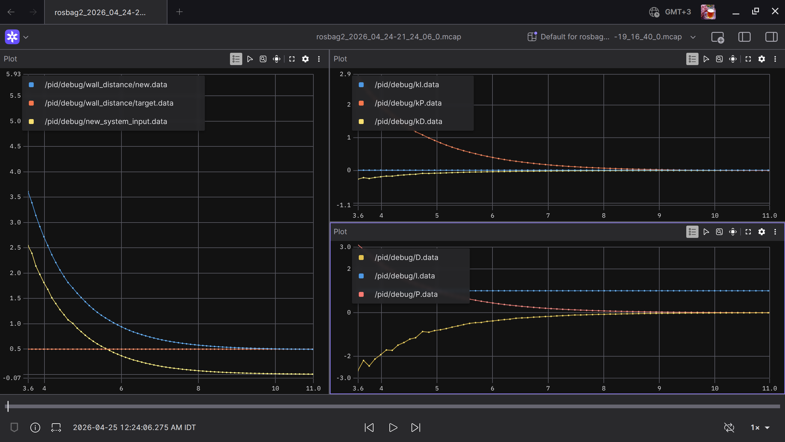
Let's break it down:
1. See the proportional part - getting smaller like in previous examples
2. See the Integral part - is being saturated, and getting winded by the Integral Winding technique
3. Observe how the Derivative part is always negative in this example, because the tracked vehicle is descending towards the wall.
Bottom Line
I can now say for sure: I "get" PID. Seeing my career and ROS intersect again was a great reminder of why I love these projects—even if it's just an hour of coding between laundry and toddlers, giving up sleep hours is worth it. This journey taught me that I've only scratched the surface of Control Theory; this field is vast. I plan to keep these PID learnings as a know-how and not dive deeper for now. But heck - this is an awesome know-how!
Cheers, Gal